White Paper - "Trading Seasonality" - The Yearly Seasonal Cycle

Introduction    What Is Seasonality?    The Yearly Seasonal Cycle
Seasonality Zones^tm    Seasonal Heat    Seasonality And Other Instruments
Deploying Seasonality As Part Of An Overall Strategy    Conclusion

There are many time periods one could use to create seasonal cycles. In fact, all cycle analysis is in reality an effort to measure seasonality. We could look at 10-year, 20-year, monthly, weekly, daily, even hourly periods in an effort to uncover repeating patterns. For the purposes of this exercise, we will focus on uncovering seasonal patterns associated with daily closing price action over the calendar year.

 

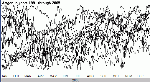
Figure 1 Amgen (AMGN) from 1991 through 2005 spliced up into yearly lines

 

Figure 1 shows the first step in preparing a seasonal cycle. We have chopped up the 15-year history of Amgen Corp (AMGN) and plotted each year starting January 1 through to the end of December. At first brush it looks like spaghetti, or for the more imaginative it might serve as some sort of Rorschach inkblot test. However, by compositing these years into one linear curve, a seasonal cycle is born.

 

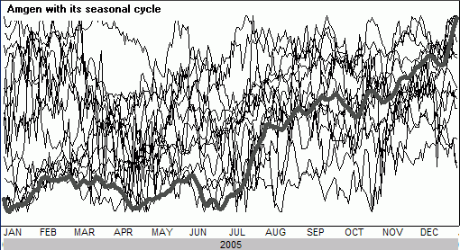
Figure 2 Amgen with its seasonal cycle

The number of years used to create a seasonal cycle is subjective. Enough years are needed to establish a statistically valuable pattern, but too many years could add old and possibly outdated information. We look back 15 years as a default, and then do a moderate process of optimization to find the best, most recent period of data to use. Optimization can be injurious to good results when testing for signals in stock data indicators. This is especially true if criteria or parameters are set as a result of excessive optimization techniques. The danger is one of curve fitting, where the indicators are parameterized to work well with a specific body of data, but are ineffective outside in the real trading world. However, here we are doing something a bit different. In any sample of data there is going to be a composite cycle. The key is to find a composite cycle that is a repeating pattern. We do this by taking a large enough sample (up to 15 years.) We then split this sample in half and create two additional composite cycles - one from the first half and one from the second half. If these two "mini" cycles are somewhat correlated, than we have greater confidence that the original cycle represents true seasonality. Optimization comes in by adjusting the original sample size to maximize the correlation of that sample's "mini" cycle halves. Let's look at an example.

 

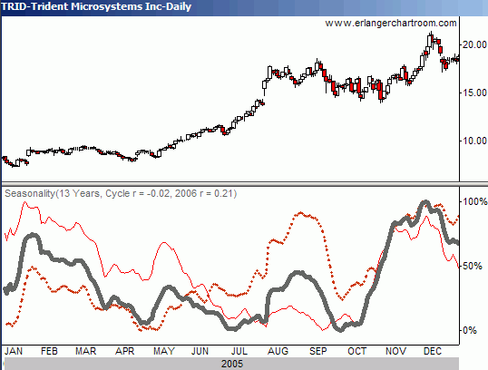
Figure 3 Trident Microsystems (TRID) with its "mini" cycles - 13 year sample

 

In Figure 3, does the seasonal pattern reflect tendencies throughout the 13-year history of Trident Microsystems (TRID), or is it a random cycle? To answer this question, we create the two "mini" seasonal composites, one from the first half of TRID's 13-year history (1993 to 1998 - see thin line in Figure 3), and one from the second half of TRID's 13-year history (1999 to 2005 - see dotted line in Figure 3.) We only use complete years in constructing seasonal cycles. If the sample size is an odd number of years, we add the median year to the latest "mini" cycle composition. The thick line is the seasonal cycle based on all 13 years of TRID price history. All these cycles bear similarities, especially at certain times of the year (the high points in late January and early December and the low point in mid-April, for instance.)

We use a correlation statistic called Pearson's R. Pearson's R is a statistical expression of linear relationship between two variables. It ranges from +1 to -1, with a reading of +1 being a perfect match between two variables. A reading of -1 indicates a perfectly inverse relationship between two variables, while a reading of 0 implies no relationship or correlation at all between the two variables. In Figure 3 in the caption is a "Cycle R^tm " statistic. This is the Pearson's R of two variables, the seasonal cycle for TRID based on years 1993 through 1998 (thin line) and the seasonal cycle for TRID based on years 1999 through 2005 (dotted line.) In this case the Cycle R^tm equals -0.02, implying no correlation. Our conclusion from this is that the yearly cycle derived from the entire 13 year history has too much noise in it to be very effective. "Noise" in the data reflects price action that is random and obscures the clarity of the seasonal pattern we are looking for. However, many of the turning points of the 13-year cycle do seem to match well with the price action in 2005. We have observed that cycles with a "Cycle R^tm " statistic around zero have some worth when looking for turning points. We eschew cycles whose "Cycle R^tm " statistic correlations are negative. These indicate a composite where conflicting patterns exist: there is too much noise in the data to expect future price action to follow the cycle.

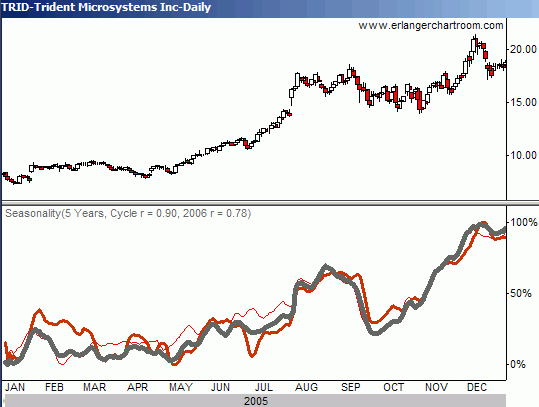
Figure 4 Microsystems (TRID) with its "mini" cycles - 5 year sample

 

Faced with a "Cycle R^tm " statistic of -0.02 for our 13-year sample cycle for TRID, we can decide to look at shorter sample periods to find a higher "Cycle r" statistic, and perhaps a more significant seasonal pattern. The sample with the highest "Cycle R^tm " statistic turns out to be of 5 years duration. Because this is a shorter sample period, the persistence of this seasonal pattern is considered to be statistically "local" - that is, less representative of longer-term cycles. Nevertheless, the trade off is a much higher "Cycle R^tm " statistic of 0.90 (see Figure 4.) In this 5-year pattern, the "mini" cycles are highly correlated. Interestingly, the key turning points found in the 13-year cycle (the high points in late January and early December and the low point in mid-April) clearly remain in the 5-year cycle.